如何在Julia中计算点积?
回字有几种写法? 🤔
两个向量$\vec{a} = [a_1, a_2, ..., a_n]$ 和 $\vec{b} = [b_1, b_2, ..., b_n]$ 之间点积(dot product)的代数定义如下:
\[\vec{a} \cdot \vec{b} = \sum^n_{i=1} a_i b_i = a_1 b_1 + a_2 b_2 + ... + a_n b_n\]
那么,如何在Julia中快速计算点积呢?
版本1: 使用 LinearAlgebra 标准库中的 dot 函数
julia> using LinearAlgebra

julia> N = 1024*1024
1048576

julia> x, y = rand(N), rand(N);

julia> dot(x,y)
262311.47579656926
先测试下标准库里 dot 的性能:
julia> using BenchmarkTools

julia> @benchmark dot($(rand(N)), $(rand(N)))
BenchmarkTools.Trial: 10000 samples with 1 evaluation.
 Range (min … max):  244.474 μs …  43.973 ms  ┊ GC (min … max): 0.00% … 0.00%
 Time  (median):     252.275 μs               ┊ GC (median):    0.00%
 Time  (mean ± σ):   314.178 μs ± 884.297 μs  ┊ GC (mean ± σ):  0.00% ± 0.00%

  ▇█▄▃▂▁▁▁▁▁▁▁ ▁▂                                               ▂
  ████████████████▇▇▇▇▇█▇▇▇▇▇▇▇▇▆▆▅▆▇▇▅▃▅▅▄▃▄▄▃▃▄▃▅▇██▆▅▅▃▄▁▃▃▃ █
  244 μs        Histogram: log(frequency) by time        594 μs <

 Memory estimate: 0 bytes, allocs estimate: 0.
中间值位于252μs附近。
版本2: for循环
当然,即使不使用自带的dot函数,我们也可以很方便地用一个 for 循环来实现:
function dot2_1(x, y)
    res = 0
    for i in eachindex(x, y)
        res += x[i] * y[i]
    end
    res
end
写法基本和原始的数学表达式一样,那性能如何呢?
julia> @benchmark dot2_1($(rand(N)), $(rand(N)))
BenchmarkTools.Trial: 2134 samples with 1 evaluation.
 Range (min … max):  2.286 ms …  2.942 ms  ┊ GC (min … max): 0.00% … 0.00%
 Time  (median):     2.302 ms              ┊ GC (median):    0.00%
 Time  (mean ± σ):   2.330 ms ± 56.418 μs  ┊ GC (mean ± σ):  0.00% ± 0.00%

  █ █
  █▃█▇▃▃▃▃▃▃▃▃▃▃▄▃▃▃▃▃▃▃▃▃▂▂▂▂▂▂▂▂▂▂▂▂▂▁▂▂▂▂▁▁▁▂▂▁▁▁▁▂▂▂▂▂▁▂ ▃
  2.29 ms        Histogram: frequency by time         2.6 ms <

 Memory estimate: 0 bytes, allocs estimate: 0.
呃, 耗时差不多是原来的9倍了。有点不可思议,那怎么优化下呢? 先用 @code_warntype 看下:
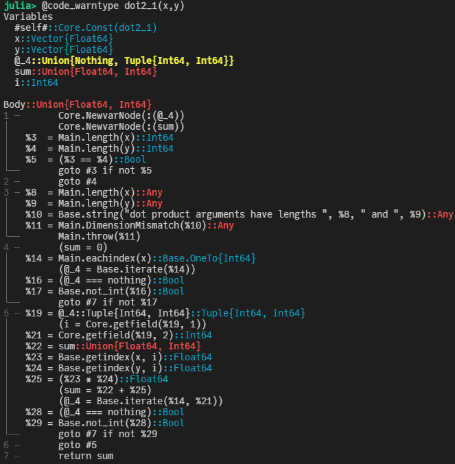
注意到上面标红色的部分,这是提醒我们上面的实现中出现了类型不稳定的情况。主要原因是res在dot2_1函数中,初始化成了Int64类型的0,而我们的输入是两个Vector{Float64}类型的向量。了解这一点之后,可以把上面的实现写得更灵活一些:
function dot2_2(x::AbstractArray{X}, y::AbstractArray{Y}) where {X,Y}
    res = zero(promote_type(X,Y))
    for i in eachindex(x, y)
        res += x[i] * y[i]
    end
    res
end
这里, 通过 promote_type 获取类型信息。
julia> @benchmark dot2_2($(rand(N)), $(rand(N)))
BenchmarkTools.Trial: 3384 samples with 1 evaluation.
 Range (min … max):  1.410 ms …  3.580 ms  ┊ GC (min … max): 0.00% … 0.00%
 Time  (median):     1.449 ms              ┊ GC (median):    0.00%
 Time  (mean ± σ):   1.464 ms ± 66.969 μs  ┊ GC (mean ± σ):  0.00% ± 0.00%

         ▆ ▃█ ▄
  ▂▃▃▃▅█▆██████▇▅█▄▄▄▄▄▄▄▃▄▄▄▃▄▄▄▄▄▃▃▄▃▃▃▂▃▃▃▂▂▃▂▂▂▂▂▁▂▂▂▂▂▂ ▃
  1.41 ms        Histogram: frequency by time        1.59 ms <

 Memory estimate: 0 bytes, allocs estimate: 0.
可以看到,比之前稍好了一些,大约是之前的5倍左右。 当然,我们还可以顺手做些进一步的优化,加上@simd并去掉边界检查:
function dot2_3(x::AbstractArray{X}, y::AbstractArray{Y}) where {X,Y}
    res = zero(promote_type(X,Y))
    @inbounds @simd for i in eachindex(x, y)
        res += x[i] * y[i]
    end
    res
end
julia> @benchmark dot2_3($(rand(N)), $(rand(N)))
BenchmarkTools.Trial: 5545 samples with 1 evaluation.
Range (min … max): 848.684 μs … 1.296 ms ┊ GC (min … max): 0.00% … 0.00%
Time (median): 871.641 μs ┊ GC (median): 0.00%
Time (mean ± σ): 888.964 μs ± 50.935 μs ┊ GC (mean ± σ): 0.00% ± 0.00%
▂▇█▇▆▇▆▅▅▅▄▄▃▃▃▂▂▁▂▁▁▁ ▂
███████████████████████▇▇▇▇▇▆▆▅▅▆▆▇█▇▇████▇█▇▅▇▇▅▅▅▄▄▅▅▅▅▅▄▃ █
849 μs Histogram: log(frequency) by time 1.11 ms <
Memory estimate: 0 bytes, allocs estimate: 0.这样差距进一步缩小了一些。当然,我们还可以进一步利用 LoopVectorization.jl 这个库来提速:
using LoopVectorization
function dot2_4(x::AbstractArray{X}, y::AbstractArray{Y}) where {X,Y}
    res = zero(promote_type(X,Y))
    @turbo for i in eachindex(x, y)
        res += x[i] * y[i]
    end
    res
end
julia> @benchmark dot2_4($(rand(N)), $(rand(N)))
BenchmarkTools.Trial: 5905 samples with 1 evaluation.
Range (min … max): 802.618 μs … 1.211 ms ┊ GC (min … max): 0.00% … 0.00%
Time (median): 820.607 μs ┊ GC (median): 0.00%
Time (mean ± σ): 832.880 μs ± 39.868 μs ┊ GC (mean ± σ): 0.00% ± 0.00%
▂█▄
▂███▆▆▇▅▄▃▃▃▃▃▂▂▂▂▂▁▁▁▁▁▁▁▁▁▁▁▁▁▁▁▁▁▁▁▁▁▁▁▁▁▁▁▁▁▁▁▁▁▁▁▁▁▁▁▁▁ ▂
803 μs Histogram: frequency by time 1.02 ms <
Memory estimate: 0 bytes, allocs estimate: 0.看起来稍微快了一些,不过似乎仍然与LinearAlgebra中的性能有3倍多的性能差距?其实不然,LinearAlgebra中使用了BLAS,而其默认是有多线程加速的,为了公平比较,可以将其线程数设置为1,然后对比:
julia> LinearAlgebra.BLAS.set_num_threads(1)

julia> @benchmark dot($(rand(N)), $(rand(N)))
BenchmarkTools.Trial: 5980 samples with 1 evaluation.
 Range (min … max):  795.374 μs …  1.104 ms  ┊ GC (min … max): 0.00% … 0.00%
 Time  (median):     811.659 μs              ┊ GC (median):    0.00%
 Time  (mean ± σ):   823.303 μs ± 37.397 μs  ┊ GC (mean ± σ):  0.00% ± 0.00%

   ▅█
  ▃███▅▇▇▅▅▄▄▄▄▃▃▃▃▃▂▂▂▂▂▂▂▂▂▂▂▂▂▂▂▂▂▂▁▂▂▂▂▂▂▂▂▂▂▂▂▂▂▂▂▂▂▂▂▂▂▂ ▃
  795 μs          Histogram: frequency by time         1.02 ms <

 Memory estimate: 0 bytes, allocs estimate: 0.
可以看到,二者相差无几。
版本3: 一行代码
当然,有的时候其实对性能也不是那么关心,反而代码的简洁性更重要,那么也可以简单地用一行代码来搞定:
julia> @benchmark sum(a*b for (a,b) in zip($(rand(N)),$(rand(N))))
BenchmarkTools.Trial: 3823 samples with 1 evaluation.
 Range (min … max):  1.232 ms …  1.840 ms  ┊ GC (min … max): 0.00% … 0.00%
 Time  (median):     1.281 ms              ┊ GC (median):    0.00%
 Time  (mean ± σ):   1.295 ms ± 54.505 μs  ┊ GC (mean ± σ):  0.00% ± 0.00%

   ▃█▇▄▆▂
  ▃███████▆▇▄▄▄▅▅▄▅▄▅▆▆▆▅▅▆▇▆▆▆▄▄▃▃▂▂▂▂▂▂▂▂▂▂▂▂▂▂▁▁▁▁▁▁▁▁▁▁▁ ▃
  1.23 ms        Histogram: frequency by time        1.46 ms <

 Memory estimate: 0 bytes, allocs estimate: 0.
或者,直接用 mapreduce:
mapreduce(*, +, x, y)版本4: 多线程
受前面LinearAlgebra中多线程的启发,我们同样也可以用Julia自带的多线程完成点积的计算。不过需要记得在启动Julia的时候,通过 -t auto 来指定线程数。
julia> using Base.Threads

julia> nthreads()
4
这里我本机就4个线程。所以
function dot4_1(x::AbstractArray{X}, y::AbstractArray{Y}) where {X,Y}
    res = zero(promote_type(X,Y))
    @threads for i in eachindex(x, y)
        res += x[i] * y[i]
    end
    res
end
julia> @benchmark dot4_1($(rand(N)), $(rand(N)))
BenchmarkTools.Trial: 109 samples with 1 evaluation.
Range (min … max): 28.586 ms … 113.851 ms ┊ GC (min … max): 0.00% … 62.77%
Time (median): 39.838 ms ┊ GC (median): 0.00%
Time (mean ± σ): 45.888 ms ± 20.565 ms ┊ GC (mean ± σ): 14.59% ± 19.04%
▁ █▃
▇█▄█▆▁▁▇██▆▇▄▄▄▁▁▁▁▁▆▁▁▁▁▁▁▁▁▁▁▁▁▁▁▁▁▁▁▁▁▁▁▁▁▁▁▁▁▁▁▄▁▁▁▄▁█▇▄ ▄
28.6 ms Histogram: log(frequency) by time 108 ms <
Memory estimate: 32.00 MiB, allocs estimate: 2097174.这个结果就比较有意思了,由于我们的多线程实现存在race condition, 实际上得到的结果并不对,并且速度相当慢。当然,为了保证结果的正确性,可以对res加锁,但并不能带来性能上的提升。一个简单的办法是,将数据分片,每个线程做自己单独的计算,最后把多个线程的结果合并:
function dot4_2(x::AbstractArray{X}, y::AbstractArray{Y}) where {X,Y}
    res = zeros(promote_type(X,Y), nthreads())
    @threads for i in 1:length(x)
        @inbounds res[threadid()] += x[i] * y[i]
    end
    sum(res)
end
julia> @benchmark dot4_2($(rand(N)), $(rand(N)))
BenchmarkTools.Trial: 10000 samples with 1 evaluation.
Range (min … max): 378.194 μs … 16.460 ms ┊ GC (min … max): 0.00% … 0.00%
Time (median): 397.990 μs ┊ GC (median): 0.00%
Time (mean ± σ): 433.403 μs ± 243.825 μs ┊ GC (mean ± σ): 0.00% ± 0.00%
▅█▆▆▆▄▂▁ ▁▁ ▁▂▂▁ ▂▃▃▂▁ ▂
██████████████▇▇███████████▇▅▆▅▅▇▅▁▃▁▃▃▁▄▁▃▁▁▅▇▄▅▃▃▄▅▄▁▄▄▆▅▄▅ █
378 μs Histogram: log(frequency) by time 878 μs <
Memory estimate: 1.98 KiB, allocs estimate: 22.这样得到的结果,相比单线程的结果要快了近3.2倍。
Julia标准库里没有提供多线程的求和操作,不过有一些第三方库提供了这类基本操作,比如ThreadsX.jl。
julia> using ThreadsX

julia> @benchmark ThreadsX.sum(a*b for (a,b) in zip($(rand(N)),$(rand(N))))
BenchmarkTools.Trial: 10000 samples with 1 evaluation.
 Range (min … max):  291.519 μs …  2.023 ms  ┊ GC (min … max): 0.00% … 0.00%
 Time  (median):     326.248 μs              ┊ GC (median):    0.00%
 Time  (mean ± σ):   339.611 μs ± 42.828 μs  ┊ GC (mean ± σ):  0.00% ± 0.00%

        ▃▆█▆▄▂▁
  ▁▂▃▅▆█████████▆▆▆▆▅▄▄▄▄▃▃▃▂▂▂▂▂▂▂▂▃▃▃▃▃▃▂▂▂▂▁▁▁▁▁▁▁▁▁▁▁▁▁▁▁▁ ▃
  292 μs          Histogram: frequency by time          472 μs <

 Memory estimate: 17.45 KiB, allocs estimate: 249.
版本5: GPU版
如果你手上正好有块GPU,不妨试试看在GPU上做点积。Julia中的CUDA.jl极大地方便了Julia语言里的GPU编程,针对点积这样的常见操作,其提供了基于cuBLAS的封装,下面来试下:
julia> using CUDA

julia> @benchmark CUDA.@sync dot($(cu(rand(N))), $(cu(rand(N))))
BenchmarkTools.Trial: 10000 samples with 1 evaluation.
 Range (min … max):  26.521 μs … 68.923 μs  ┊ GC (min … max): 0.00% … 0.00%
 Time  (median):     27.798 μs              ┊ GC (median):    0.00%
 Time  (mean ± σ):   28.331 μs ±  1.494 μs  ┊ GC (mean ± σ):  0.00% ± 0.00%

  ▂▁   ▃▇█▅▁ ▃▅▇▅▂   ▂▃                                       ▂
  ███▆▇████████████▇████▆▄▄▅▆▆▅▅▅▅▅▅▅▆▆▆▆▅▆▄▅▆▅▄▅▅▂▅▄▄▅▅▄▄▃▅▄ █
  26.5 μs      Histogram: log(frequency) by time      35.9 μs <

 Memory estimate: 16 bytes, allocs estimate: 1.
可以看到,其速度相当快。
不过,由于cuBLAS里的dot只针对常见的 Float32, Float64, Float16 以及对应的复数类型的GPU上的向量有实现,当输入的两个向量的元素类型不一致时,目前的CUDA.jl(v3.5.0)会fallback到CPU版本的实现,导致性能极慢:
julia> z = rand(Bool, N);

julia> cx, cz = cu(x), cu(z);

julia> @time dot(cx, cz)
┌ Warning: Performing scalar indexing on task Task (runnable) @0x00007f63cc0c0010.
│ Invocation of getindex resulted in scalar indexing of a GPU array.
│ This is typically caused by calling an iterating implementation of a method.
│ Such implementations *do not* execute on the GPU, but very slowly on the CPU,
│ and therefore are only permitted from the REPL for prototyping purposes.
│ If you did intend to index this array, annotate the caller with @allowscalar.
└ @ GPUArrays ~/.julia/packages/GPUArrays/3sW6s/src/host/indexing.jl:56
12.914170 seconds (6.29 M allocations: 1.000 GiB, 0.87% gc time)一个简单的workaround是,先把类型不同的两个向量转换成相同的类型,然后再调用dot函数:
julia> @benchmark CUDA.@sync dot($(cu(rand(N))), convert(CuArray{Float32}, $(cu(rand(Bool, N)))))
BenchmarkTools.Trial: 3968 samples with 1 evaluation.
 Range (min … max):  1.073 ms …   4.408 ms  ┊ GC (min … max): 0.00% … 30.06%
 Time  (median):     1.140 ms               ┊ GC (median):    0.00%
 Time  (mean ± σ):   1.252 ms ± 464.709 μs  ┊ GC (mean ± σ):  3.35% ±  6.05%

  ▂█▃  ▄▁                                     ▁
  ███▇▆██▆▄▁▁▁▁▁▁▁▁▁▁▁▁▁▁▁▁▁▁▁▁▁▁▁▁▁▁▁▁▁▁▁▁▁▁▄█▅▃▁▃▁▁▁▃▁▃▁▁▁█ █
  1.07 ms      Histogram: log(frequency) by time      3.85 ms <

 Memory estimate: 5.00 MiB, allocs estimate: 12.
相比原来的GPU版本,多出来了一次拷贝数据的时间,这显然不是我们想要的。 不过,CUDA.jl的强大之处在于,针对这类没有内置的实现,我们可以很容易地通过编写自定义的核函数来实现。
function dot5_1(x::CuArray{T1}, y::CuArray{T2}) where {T1, T2}
    T = promote_type(T1, T2)
    res = CuArray{T}([zero(T)])
    function kernel(x, y, res)
        for i in 1:length(x)
            @inbounds res[] += x[i] * y[i]
        end
    end
    @cuda kernel(x, y, res)
    res[]
end
自己手写核函数经常容易出现各种bug,所以首要任务是先确认我们计算的结果是正确的:
julia> isapprox(dot5_1(cx, cz), dot(cx, convert(CuArray{Float32}, cz)))
true注意这里用的是isapprox来做比较。看起来我们得到的结果是正确的,那么其性能如何呢?
julia> @benchmark CUDA.@sync dot5_1($(cu(rand(N))), $(cu(rand(Bool, N))))
BenchmarkTools.Trial: 103 samples with 1 evaluation.
 Range (min … max):  48.510 ms …  54.895 ms  ┊ GC (min … max): 0.00% … 0.00%
 Time  (median):     48.514 ms               ┊ GC (median):    0.00%
 Time  (mean ± σ):   48.606 ms ± 657.494 μs  ┊ GC (mean ± σ):  0.00% ± 0.00%

  █▁
  ███▁▁▄▁▁▁▁▁▁▁▁▁▁▁▁▁▁▁▁▁▁▁▁▁▁▁▁▁▁▁▁▁▁▁▁▁▁▁▁▁▁▁▁▁▁▁▁▁▁▁▁▁▁▁▁▁▄ ▄
  48.5 ms       Histogram: log(frequency) by time      50.6 ms <

Memory estimate: 1.78 KiB, allocs estimate: 29.呃,还不如先convert了再调用自带的dot函数...... 那问题出在哪呢?其实上面的核函数只用了一个线程在计算,但是在GPU上有大量的线程可供计算,于是,可以采用上面的CPU上多线程的方法来计算:
function dot5_2(x::CuArray{T1}, y::CuArray{T2}) where {T1, T2}
    T = promote_type(T1, T2)
    res = CuArray{T}([zero(T)])
    function kernel(x, y, res)
        index = threadIdx().x
        stride = blockDim().x
        for i in index:stride:length(x)
            @inbounds res[] += x[i] * y[i]
        end
    end
    k = @cuda launch=false kernel(x, y, res)
    config = launch_configuration(k.fun)
    k(x, y, res; threads=min(length(x), config.threads))
    CUDA.@allowscalar res[]
end这里在运行核函数的时候,指定了threads的个数,在核函数内部的for循环把数据根据threads切分成了不同的片段,每个thread负责计算各自的一部分。 先验证下正确性:
julia> isapprox(dot5_2(cx, cz), dot(cx, convert(CuArray{Float32}, cz)))
false等等,这里似乎犯了和前面多线程计算时候一样的错误,在往res里累积求和的时候,会存在静态条件。仔细观察可以发现,我们不用每次都往res里写入结果,只需要在每个线程内部先计算完,最后叠加上去即可,同时最后要加锁。
function dot5_3(x::CuArray{T1}, y::CuArray{T2}) where {T1, T2}
    T = promote_type(T1, T2)
    res = CuArray{T}([zero(T)])
    function kernel(x, y, res, T)
        index = threadIdx().x
        stride = blockDim().x
        s = zero(T)
        for i in index:stride:length(x)
            @inbounds s += x[i] * y[i]
        end
        CUDA.@atomic res[] += s
        return nothing
    end
    k = @cuda launch=false kernel(x, y, res,T)
    config = launch_configuration(k.fun)
    k(x, y, res, T; threads=min(length(x), config.threads))
    CUDA.@allowscalar res[]
end这里用了CUDA.@atomic来保证原子操作,同样,先确认计算的正确性:
julia> isapprox(dot(cx, cz), dot5_3(cx, cz))
true
再看下速度如何:
julia> @benchmark CUDA.@sync dot5_3($(cu(rand(N))), $(cu(rand(Bool, N))))
BenchmarkTools.Trial: 10000 samples with 1 evaluation.
 Range (min … max):  175.298 μs … 448.774 μs  ┊ GC (min … max): 0.00% … 0.00%
 Time  (median):     178.373 μs               ┊ GC (median):    0.00%
 Time  (mean ± σ):   179.218 μs ±   4.301 μs  ┊ GC (mean ± σ):  0.00% ± 0.00%

    ▁▃▅▅▇█████▇▇▇▇▇▆▆▅▅▄▄▃▂▂▁▁▁▁ ▁   ▁▁▁▁▁ ▁▁▁▁▁▁▁              ▃
  ▅▅██████████████████████████████████████████████▇██▇▇▆▇▆▅▅▇▅▆ █
  175 μs        Histogram: log(frequency) by time        191 μs <

 Memory estimate: 2.16 KiB, allocs estimate: 39.
还不错,至少比CPU版本快了,但是离CUBLAS版本的性能还有一定差距。
考虑到一块GPU中,还会有多个block,而上面我们才用了其中的一个block,显然还有很大的优化空间!
一个基本思路是,根据输入的数据,分配多个block,在每个block的数据区块中,按thread再切分一次,每个thread计算自己所属的数据的点积之和。
function dot5_4(x::CuArray{T1}, y::CuArray{T2}) where {T1, T2}
    T = promote_type(T1, T2)
    res = CuArray{T}([zero(T)])
    function kernel(x, y, res, T)
        index = threadIdx().x
        thread_stride = blockDim().x
        block_stride = (length(x)-1) ÷ gridDim().x + 1
        start = (blockIdx().x - 1) * block_stride + 1
        stop = blockIdx().x * block_stride

        s = zero(T)
        for i in start-1+index:thread_stride:stop
            @inbounds s += x[i] * y[i]
        end
        CUDA.@atomic res[] += s
        return nothing
    end
    k = @cuda launch=false kernel(x, y, res,T)
    config = launch_configuration(k.fun)
    k(x, y, res, T; threads=min(length(x), config.threads), blocks=config.blocks)
    CUDA.@allowscalar res[]
end
julia> isapprox(dot(cx, cz), dot5_4(cx, cz))
true
julia> @benchmark CUDA.@sync dot5_4($(cu(rand(N))), $(cu(rand(Bool, N))))
BenchmarkTools.Trial: 10000 samples with 1 evaluation.
Range (min … max): 134.011 μs … 383.172 μs ┊ GC (min … max): 0.00% … 0.00%
Time (median): 134.933 μs ┊ GC (median): 0.00%
Time (mean ± σ): 135.095 μs ± 2.723 μs ┊ GC (mean ± σ): 0.00% ± 0.00%
▁▃▄▇▇▇▆████▇▆▃▃▁
▂▂▃▅▆█████████████████▆▅▅▅▄▃▃▃▃▃▂▂▂▂▂▂▂▂▂▂▂▂▂▂▂▂▂▂▂▂▂▂▂▂▁▂▂▂▂ ▄
134 μs Histogram: frequency by time 138 μs <
Memory estimate: 2.16 KiB, allocs estimate: 39.OK, 看起来稍微快了一些。需要注意的是,前面我们直接将每个thread计算的结果往一个res对象中通过加锁叠加上去了,这样导致每个block中每个thread都会卡在原子操作那一步。 一种优化方式是每个block的内部,先把各个thread的计算结果缓存起来,等一个block内所有thread都计算出来了同步一下,然后内部先reduce,最后再通过原子操作同步到最终的结果上。
function dot5_5(x::CuArray{T1}, y::CuArray{T2}) where {T1, T2}
    T = promote_type(T1, T2)
    res = CuArray{T}([zero(T)])
    function kernel(x, y, res, T)
        index = threadIdx().x
        thread_stride = blockDim().x
        block_stride = (length(x)-1) ÷ gridDim().x + 1
        start = (blockIdx().x - 1) * block_stride + 1
        stop = blockIdx().x * block_stride

        cache = CuDynamicSharedArray(T, (thread_stride,))

        for i in start-1+index:thread_stride:stop
            @inbounds cache[index] += x[i] * y[i]
        end

        sync_threads()

        if index == 1
            s = zero(T)
            for i in 1:thread_stride
                s += cache[i]
            end
            CUDA.@atomic res[] += s
        end
        return nothing
    end
    k = @cuda launch=false kernel(x, y, res,T)
    config = launch_configuration(k.fun; shmem=(threads) -> threads*sizeof(T))
    threads = min(length(x), config.threads)
    blocks = config.blocks
    k(x, y, res, T; threads=threads, blocks=config.blocks, shmem=threads*sizeof(T))
    CUDA.@allowscalar res[]
end
julia> isapprox(dot(cx, cz), dot5_5(cx, cz))
true
julia> @benchmark CUDA.@sync dot5_5($(cu(rand(N))), $(cu(rand(Bool, N))))
BenchmarkTools.Trial: 10000 samples with 1 evaluation.
Range (min … max): 54.364 μs … 358.597 μs ┊ GC (min … max): 0.00% … 0.00%
Time (median): 55.217 μs ┊ GC (median): 0.00%
Time (mean ± σ): 55.559 μs ± 4.023 μs ┊ GC (mean ± σ): 0.00% ± 0.00%
▄▇█▇▅▃▂
▂▄█████████▇▇▆▅▄▄▃▃▃▃▃▃▂▂▂▂▂▂▂▂▂▂▂▂▂▂▂▂▂▂▂▂▂▂▂▂▂▂▂▂▂▂▂▂▂▁▂▁▂ ▃
54.4 μs Histogram: frequency by time 61.3 μs <
Memory estimate: 2.33 KiB, allocs estimate: 43.可以看到,其性能跟CUBLAS比较接近了。当然,上面的代码还可以进一步优化,上面最后reduce的时候,只有index为1的线程在运行,其实可以多个线程一起工作:
using CUDA:i32

function dot5_6(x::CuArray{T1}, y::CuArray{T2}) where {T1, T2}
    T = promote_type(T1, T2)
    res = CuArray{T}([zero(T)])
    function kernel(x, y, res, T)
        index = threadIdx().x
        thread_stride = blockDim().x
        block_stride = (length(x)-1i32) ÷ gridDim().x + 1i32
        start = (blockIdx().x - 1i32) * block_stride + 1i32
        stop = blockIdx().x * block_stride

        cache = CuDynamicSharedArray(T, (thread_stride,))

        for i in start-1i32+index:thread_stride:stop
            @inbounds cache[index] += x[i] * y[i]
        end
        sync_threads()

        mid = thread_stride
        while true
            mid = (mid - 1i32) ÷ 2i32 + 1i32
            if index <= mid
                @inbounds cache[index] += cache[index+mid]
            end
            sync_threads()
            mid == 1i32 && break
        end

        if index == 1i32
            CUDA.@atomic res[] += cache[1]
        end
        return nothing
    end
    k = @cuda launch=false kernel(x, y, res,T)
    config = launch_configuration(k.fun; shmem=(threads) -> threads*sizeof(T))
    threads = min(length(x), config.threads)
    blocks = config.blocks
    k(x, y, res, T; threads=threads, blocks=config.blocks, shmem=threads*sizeof(T))
    CUDA.@allowscalar res[]
end
julia> isapprox(dot(cx, cz), dot5_6(cx, cz))
true
julia> @benchmark CUDA.@sync dot5_6($(cu(rand(N))), $(cu(rand(Bool, N))))
BenchmarkTools.Trial: 10000 samples with 1 evaluation.
Range (min … max): 22.520 μs … 375.954 μs ┊ GC (min … max): 0.00% … 0.00%
Time (median): 23.475 μs ┊ GC (median): 0.00%
Time (mean ± σ): 23.762 μs ± 3.748 μs ┊ GC (mean ± σ): 0.00% ± 0.00%
▁▅██▆▃▁
▂▂▃▃▄▆███████▇▅▄▅▅▅▆▅▄▄▃▃▃▂▂▂▂▂▂▂▂▂▁▂▂▁▂▂▂▂▂▂▂▂▁▂▂▂▂▂▂▂▂▁▂▂▂ ▃
22.5 μs Histogram: frequency by time 28 μs <
Memory estimate: 2.16 KiB, allocs estimate: 39.这样,最终的结果跟CUBLAS的性能基本一致了。
从代码层面上讲,上面的代码还可以进一步简化下,上面的while循环其实是一个经典的reduce操作,而CUDA.jl中内置了一个函数reduce_block来简化该操作,下面是简化后的核函数写法:
    function kernel(x, y, res::AbstractArray{T}, shuffle) where {T}
        local_val = zero(T)

        # grid-stride loop
        i = threadIdx().x + (blockIdx().x - 1i32)*blockDim().x
        while i <= length(x)
            @inbounds local_val += dot(x[i], y[i])
            i += blockDim().x * gridDim().x
        end

        val = reduce_block(+, local_val, zero(T), shuffle)
        if threadIdx().x == 1i32
            # NOTE: introduces nondeterminism
            @inbounds @atomic res[] += val
        end

        return
end忘了说了,如果你还是one-line solution的爱好者,其实之前的CPU版本的写法在GPU上同样work哦~
mapreduce((x,y)->dot(x, y), +, x, y)